Arrays of Wisdom of the Ancients

Aleksey Shipilёv, @shipilev, aleksey@shipilev.net

This post is also available in ePUB and mobi.

Thanks to Claes Redestad, Brian Goetz, Ilya Teterin, Yurii Lahodiuk, Gleb Smirnov, Tim Ellison, Stuart Marks, Marshall Pierce, Fabian Lange and others for reviews and helpful suggestions!

Introduction

The Java Language and JDK Class Library have two distinct, yet connected, ways to group elements: arrays and Collections. There are pros and cons for using either one, so both are prevalent in real programs. To aid conversion between the two, there are standard methods to make a reference array appear as a Collection (e.g. Arrays.asList), and to copy from Collection to array (e.g. several Collection.toArray methods). In this post, we will try to answer a controversial question: which toArray conversion pattern is faster?

The post uses JMH as the research crucible. If you haven’t learned about it yet, and/or haven’t looked through the JMH samples, I suggest you do that before reading the rest of this post for the best experience. Some x86 assembly knowledge is also helpful, though not strictly required.

This post is long and may be very tough for beginners, because it touches on many different things, and has several subflows. I could have split it into the several posts, but I tried, and it turned out messy. If you start to lose a flow, bookmark the post, and resume reading after some rest!

API Design

It seems very natural to call toArray blindly on a Collection, and/or follow whatever advice we can find with tools, or with frantic internet searches. But if we look at the Collection.toArray family of methods, we can see two separate methods:

public interface Collection<E> extends Iterable<E> {

    /**
     * Returns an array containing all of the elements in this collection.
     *
     * ...
     *
     * @return an array containing all of the elements in this collection
     */
    Object[] toArray();

    /**
     * Returns an array containing all of the elements in this collection;
     * the runtime type of the returned array is that of the specified array.
     * If the collection fits in the specified array, it is returned therein.
     * Otherwise, a new array is allocated with the runtime type of the
     * specified array and the size of this collection.
     *
     * ...
     *
     * @param <T> the runtime type of the array to contain the collection
     * @param a the array into which the elements of this collection are to be
     *        stored, if it is big enough; otherwise, a new array of the same
     *        runtime type is allocated for this purpose.
     * @return an array containing all of the elements in this collection
     * @throws ArrayStoreException if the runtime type of the specified array
     *         is not a supertype of the runtime type of every element in
     *         this collection
     */
    <T> T[] toArray(T[] a);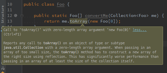

Figure 1. IntelliJ IDEA 15 tries to help us

Figure 2. PMD 5.4.1 tries to help me

These methods behave subtly differently, and for a reason. The impedance caused by type erasure in generics forces us to spell out the target array type exactly using the actual argument. Note that simply casting the Object[] returned from toArray() to ConcreteType[] would not work, because the runtime has to maintain type safety — trying to cast the array like that will result in a ClassCastException. This secures from a malicious code that could try to circumvent type safety by putting something non-ConcreteType into that Object[] array.

The array-accepting method can also be used to pass through a pre-allocated array in which to put the results. In fact, the wisdom of the ancients might be trying to tell us we are much better off providing the pre-sized array (may be even zero-sized!), for best performance. IntelliJ IDEA 15 suggests passing the pre-sized array, instead of being lazy and passing a zero-sized array. It goes on to explain that a library would have to do a reflection call to allocate the array of a given runtime type, and that apparently costs you.

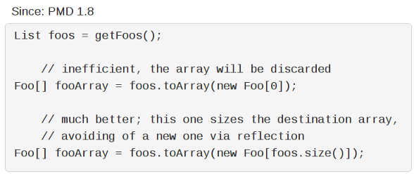
PMD’s OptimizableToArrayCall rule tells us the same, but also seems to imply that a newly-allocated "empty" array would be discarded, and we should avoid that by passing a pre-sized destination array.

How smart are the ancients really?

Performance Runs

Experimental Setup

Before we conduct the experiment, we need to understand the degrees of freedom. There are at least three to consider:

Collection size. PMD’s rule suggests that allocating the array that is going to be discarded is futile. This means we want to cover a number of small collection sizes to see the impact of "gratuitous" array instantiations. We would also like to see how large collections perform, when we would expect element copying costs to dominate. Naturally, we want to prod the sizes in between in order to avoid "performance sweet spots".
toArray() argument shapes. Of course, we want to try all variants of toArray calls. The particular interest is the zero-sized-array call vs. the presized-array call, but a non-typed toArray is also interesting as a reference.
toArray() implementations in Collections. IDEA suggests there is a possible reflective array instantiation that costs performance. We need to investigate what collections are actually using. Most collections do the same as AbstractCollection : allocate either an Object[] or a T[] array — in the latter case, indeed, allocating the T[] array using the java.lang.reflect.Array::newInstance method — then picking up the iterator, and copying the elements one-by-one into the destination array.
```
public abstract class AbstractCollection {
  public <T> T[] toArray(T[] a) {
    int size = size();
    T[] r = (a.length >= size) ?
             a : (T[])Array.newInstance(a.getClass().getComponentType(), size);
    Iterator<E> it = iterator();
    for (int i = 0; i < r.length; i++) {
      ...
      r[i] = (T)it.next();
    }
    return ... r;
  }
}
```
Some collections, notably ArrayList, simply copy their backing array storage to the destination array:
```
public class ArrayList {
  public <T> T[] toArray(T[] a) {
    if (a.length < size) {
      // Arrays.copyOf would do the Array.newInstance
      return (T[]) Arrays.copyOf(elementData, size, a.getClass());
    }
    System.arraycopy(elementData, 0, a, 0, size);
    if (a.length > size) {
      a[size] = null;
    }
    return a;
  }
}
```
ArrayList is one of the most frequently used collection classes, and so we would want to see how both a ubiquitous ArrayList, and a generic, AbstractCollection-backed collection like HashSet perform.

Benchmark

With the observations from above, we can construct the following JMH benchmark:

@Warmup(iterations = 5, time = 1, timeUnit = TimeUnit.SECONDS)
@Measurement(iterations = 5, time = 1, timeUnit = TimeUnit.SECONDS)
@Fork(value = 3, jvmArgsAppend = {"-XX:+UseParallelGC", "-Xms1g", "-Xmx1g"})
@BenchmarkMode(Mode.AverageTime)
@OutputTimeUnit(TimeUnit.NANOSECONDS)
@State(Scope.Benchmark)
public class ToArrayBench {

    @Param({"0", "1", "10", "100", "1000"})
    int size;

    @Param({"arraylist", "hashset"})
    String type;

    Collection<Foo> coll;

    @Setup
    public void setup() {
        if (type.equals("arraylist")) {
            coll = new ArrayList<Foo>();
        } else if (type.equals("hashset")) {
            coll = new HashSet<Foo>();
        } else {
            throw new IllegalStateException();
        }
        for (int i = 0; i < size; i++) {
            coll.add(new Foo(i));
        }
    }

    @Benchmark
    public Object[] simple() {
        return coll.toArray();
    }

    @Benchmark
    public Foo[] zero() {
        return coll.toArray(new Foo[0]);
    }

    @Benchmark
    public Foo[] sized() {
        return coll.toArray(new Foo[coll.size()]);
    }

    public static class Foo {
        private int i;

        public Foo(int i) {
            this.i = i;
        }

        @Override
        public boolean equals(Object o) {
            if (this == o) return true;
            if (o == null || getClass() != o.getClass()) return false;
            Foo foo = (Foo) o;
            return i == foo.i;
        }

        @Override
        public int hashCode() {
            return i;
        }
    }
}

Since this benchmark is GC-intensive, it is important to fix the GC algorithm and heap sizes to avoid surprises with heuristics that may change behavior unexpectedly. This is especially important for comparisons between JDK versions, and for benchmarks that incur lots of allocations. Note how we lock down Parallel GC, with static 1 Gb heap with a @Fork annotation above.

Performance Data

Running on quite a large i7-4790K, 4.0 GHz, Linux x86_64, JDK 9b99 EA, will yield (average execution time, the lower the better):

Benchmark            (size)     (type)  Mode  Cnt      Score    Error  Units

# ---------------------------------------------------------------------------

ToArrayBench.simple       0  arraylist  avgt   30    19.445 ±   0.152  ns/op
ToArrayBench.sized        0  arraylist  avgt   30    19.009 ±   0.252  ns/op
ToArrayBench.zero         0  arraylist  avgt   30     4.590 ±   0.023  ns/op

ToArrayBench.simple       1  arraylist  avgt   30     7.906 ±   0.024  ns/op
ToArrayBench.sized        1  arraylist  avgt   30    18.972 ±   0.357  ns/op
ToArrayBench.zero         1  arraylist  avgt   30    10.472 ±   0.038  ns/op

ToArrayBench.simple      10  arraylist  avgt   30     8.499 ±   0.049  ns/op
ToArrayBench.sized       10  arraylist  avgt   30    24.637 ±   0.128  ns/op
ToArrayBench.zero        10  arraylist  avgt   30    15.845 ±   0.075  ns/op

ToArrayBench.simple     100  arraylist  avgt   30    40.874 ±   0.352  ns/op
ToArrayBench.sized      100  arraylist  avgt   30    93.170 ±   0.379  ns/op
ToArrayBench.zero       100  arraylist  avgt   30    80.966 ±   0.347  ns/op

ToArrayBench.simple    1000  arraylist  avgt   30   400.130 ±   2.261  ns/op
ToArrayBench.sized     1000  arraylist  avgt   30   908.007 ±   5.869  ns/op
ToArrayBench.zero      1000  arraylist  avgt   30   673.682 ±   3.586  ns/op

# ---------------------------------------------------------------------------

ToArrayBench.simple       0    hashset  avgt   30    21.270 ±   0.424  ns/op
ToArrayBench.sized        0    hashset  avgt   30    20.815 ±   0.400  ns/op
ToArrayBench.zero         0    hashset  avgt   30     4.354 ±   0.014  ns/op

ToArrayBench.simple       1    hashset  avgt   30    22.969 ±   0.221  ns/op
ToArrayBench.sized        1    hashset  avgt   30    23.752 ±   0.503  ns/op
ToArrayBench.zero         1    hashset  avgt   30    23.732 ±   0.076  ns/op

ToArrayBench.simple      10    hashset  avgt   30    39.630 ±   0.613  ns/op
ToArrayBench.sized       10    hashset  avgt   30    43.808 ±   0.629  ns/op
ToArrayBench.zero        10    hashset  avgt   30    44.192 ±   0.823  ns/op

ToArrayBench.simple     100    hashset  avgt   30   298.032 ±   3.925  ns/op
ToArrayBench.sized      100    hashset  avgt   30   316.250 ±   9.614  ns/op
ToArrayBench.zero       100    hashset  avgt   30   284.431 ±   6.201  ns/op

ToArrayBench.simple    1000    hashset  avgt   30  4227.564 ±  84.983  ns/op
ToArrayBench.sized     1000    hashset  avgt   30  4539.614 ± 135.379  ns/op
ToArrayBench.zero      1000    hashset  avgt   30  4428.601 ± 205.191  ns/op

# ---------------------------------------------------------------------------

Okay, it appears that a simple conversion wins over everything else, and, counter-intuitively, zero conversion wins over sized.

At this point, most people make the major mistake: they run with these numbers as if they are the truth. But these numbers are just data, they don’t mean anything unless we extract the insights out of them. To do that, we need to see why the numbers are like that.

Looking closely at the data, we want to get the answers on two major questions:

Why does simple appear faster than zero and sized?
Why does zero appear faster than sized?

Answering these questions is the road to understanding what is going on.

The running exercise for any good performance engineer would be to try to guess the answers before starting the investigation to figure out the actual ones, thus training the intuition. Take a few minutes to come up with plausible hypothetical answers to these questions. What experiments would you have to do to confirm the hypotheses? What experiments would be able to falsify them?

Not an Allocation Pressure

I’d like to throw out a simple hypothesis though: allocation pressure. One might speculate that different allocation pressures can explain the difference in performance. In fact, many GC-intensive workloads are also GC-bound, meaning the benchmark performance is tidally locked with GC performance.

It is usually easy to turn quite a few benchmarks into GC-bound ones. In our case, we are running the benchmark code with a single thread, which leaves GC threads free to run on separate cores, picking up the single benchmark thread’s garbage with multiple GC threads. Adding more benchmark threads will make them: a) compete with GC threads for CPU time, thus implicitly counting in the GC time, and b) produce much more garbage, so that the effective number of GC threads per application thread goes down, exacerbating the memory management costs.

This is one of the reasons why you would normally want to run benchmarks in both single-threaded and multi-threaded (saturated) modes. Running in saturated mode captures whatever "hidden" offload activity the system is doing.

But, in our case, we can take a shortcut and estimate the allocation pressure directly. For that, JMH has the -prof gc profiler, that listens for GC events, adds them up, and normalizes the allocation/churn rates to the number of benchmark ops, giving you the allocation pressure per @Benchmark call.

Allocation pressure (the table shows only "gc.alloc.rate.norm" metric)

Benchmark           (size)     (type)  Mode  Cnt    Score    Error  Units

# ------------------------------------------------------------------------

ToArrayBench.simple      0  arraylist  avgt   30    16.000 ± 0.001  B/op
ToArrayBench.sized       0  arraylist  avgt   30    16.000 ± 0.001  B/op
ToArrayBench.zero        0  arraylist  avgt   30    16.000 ± 0.001  B/op

ToArrayBench.simple      1  arraylist  avgt   30    24.000 ± 0.001  B/op
ToArrayBench.sized       1  arraylist  avgt   30    24.000 ± 0.001  B/op
ToArrayBench.zero        1  arraylist  avgt   30    40.000 ± 0.001  B/op

ToArrayBench.simple     10  arraylist  avgt   30    56.000 ± 0.001  B/op
ToArrayBench.sized      10  arraylist  avgt   30    56.000 ± 0.001  B/op
ToArrayBench.zero       10  arraylist  avgt   30    72.000 ± 0.001  B/op

ToArrayBench.simple    100  arraylist  avgt   30   416.000 ± 0.001  B/op
ToArrayBench.sized     100  arraylist  avgt   30   416.000 ± 0.001  B/op
ToArrayBench.zero      100  arraylist  avgt   30   432.000 ± 0.001  B/op

ToArrayBench.simple   1000  arraylist  avgt   30  4016.001 ± 0.001  B/op
ToArrayBench.sized    1000  arraylist  avgt   30  4016.001 ± 0.002  B/op
ToArrayBench.zero     1000  arraylist  avgt   30  4032.001 ± 0.001  B/op

# ------------------------------------------------------------------------

ToArrayBench.simple      0    hashset  avgt   30    16.000 ± 0.001  B/op
ToArrayBench.sized       0    hashset  avgt   30    16.000 ± 0.001  B/op
ToArrayBench.zero        0    hashset  avgt   30    16.000 ± 0.001  B/op

ToArrayBench.simple      1    hashset  avgt   30    24.000 ± 0.001  B/op
ToArrayBench.sized       1    hashset  avgt   30    24.000 ± 0.001  B/op
ToArrayBench.zero        1    hashset  avgt   30    24.000 ± 0.001  B/op

ToArrayBench.simple     10    hashset  avgt   30    56.000 ± 0.001  B/op
ToArrayBench.sized      10    hashset  avgt   30    56.000 ± 0.001  B/op
ToArrayBench.zero       10    hashset  avgt   30    56.000 ± 0.001  B/op

ToArrayBench.simple    100    hashset  avgt   30   416.000 ± 0.001  B/op
ToArrayBench.sized     100    hashset  avgt   30   416.001 ± 0.001  B/op
ToArrayBench.zero      100    hashset  avgt   30   416.001 ± 0.001  B/op

ToArrayBench.simple   1000    hashset  avgt   30  4056.006 ± 0.009  B/op
ToArrayBench.sized    1000    hashset  avgt   30  4056.007 ± 0.010  B/op
ToArrayBench.zero     1000    hashset  avgt   30  4056.006 ± 0.009  B/op

# ------------------------------------------------------------------------

The data indeed show that allocation pressure is mostly the same within the same size. zero tests are allocating 16 bytes more in some cases — that’s the cost for "redundant" array allocation. (Exercise for the readers: why it is the same for zero with hashset cases?). But, our throughput benchmarks above suggests that zero cases are faster, not slower, as the allocation pressure hypothesis would predict. Therefore, allocation pressure cannot be the explanation for the phenomenon we are seeing.

Performance Analysis

In our field, we can skip the hypotheses building and go straight to poking the stuff with power tools. This section could be shorter, if we used hindsight, and breezed straight to the conclusion. But one of the points for this post is to show off the approaches one can take to analyze these benchmarks.

Meet VisualVM (and other Java-only profilers)

The most obvious approach is to attach a Java profiler to the benchmarked JVM, and see what is going on there. Without loss of generality, let’s take the VisualVM profiler that is shipped with JDK itself, and thus readily available on most installations.

It is very easy to use: start the application, start VisualVM (if the JDK is in your PATH, then invoking jvisualvm is enough), select a target VM from the list, select "Sample" from a drop-down list or a tab, press the "CPU Sampling" button, and enjoy the results. Let’s take one of our tests and see what it shows us:

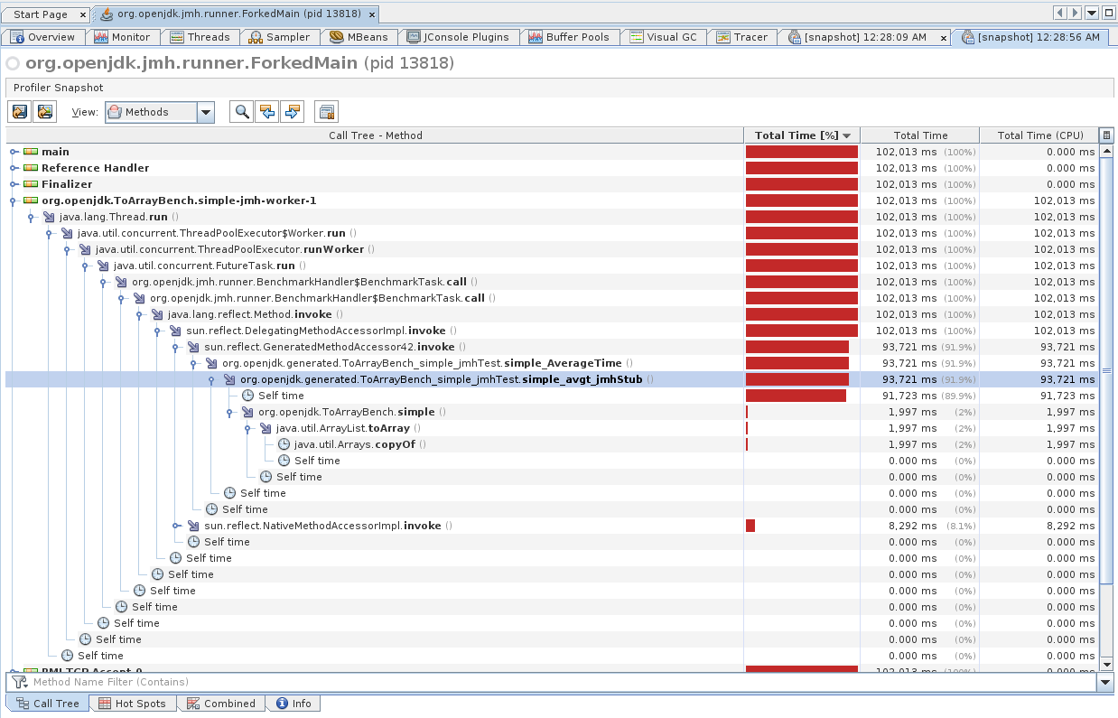
Figure 3. VisualVM profile snapshot for the "ToArrayBench.simple" case and ArrayList of size 1000

Err… Very informative.

Most Java profilers are inherently biased, because they either instrument the code and thus offset the real results, or they sample at designated places in the code (e.g. safepoints) that also skews the results. In our case above, while the bulk of work is done in simple() method, profiler misattributes the work to …_jmhStub method that holds the benchmark loop.

But this is not the central issue here. The most problematic part for us is the absence of any low-level details that may help us to answer performance questions. Can you see anything in the profiling snapshot above that can verify any sensible hypothesis in our case? You cannot, because the data is too coarse. Note that this is not an issue for larger workloads where performance phenomena manifest in larger and more distributed call trees. In those workloads, bias effects are smoothed out.

Meet JMH -prof perfasm

The need to explore low-level details for microbenchmarks is the reason why good microbenchmark harnesses provide a clear-cut way to profile, analyze, and introspect tiny workloads. In case of JMH, we have the embedded "perfasm" profiler that dumps PrintAssembly output from the VM, annotates it with perf_events counters, and prints out the hottest parts. perf_events provides non-intrusive sampling profiling with hardware counters, which is what we want for fine-grained performance engineering.

Below is the example output for one of the tests:

$ java -jar target/benchmarks.jar zero -f 1 -p size=1000 -p type=arraylist -prof perfasm
....[Hottest Region 1].......................................................................
 [0x7fc4c180916e:0x7fc4c180920c] in StubRoutines::checkcast_arraycopy

StubRoutines::checkcast_arraycopy [0x00007fc4c18091a0, 0x00007fc4c180926b]
  0.04%                  0x00007fc4c18091a0: push   %rbp
  0.06%    0.01%         0x00007fc4c18091a1: mov    %rsp,%rbp
  0.01%                  0x00007fc4c18091a4: sub    $0x10,%rsp
  0.02%    0.01%         0x00007fc4c18091a8: mov    %r13,(%rsp)
  0.14%    0.02%         0x00007fc4c18091ac: mov    %r14,0x8(%rsp)
  0.07%    0.02%         0x00007fc4c18091b1: lea    (%rdi,%rdx,4),%rdi
  0.01%                  0x00007fc4c18091b5: lea    (%rsi,%rdx,4),%r13
                         0x00007fc4c18091b9: mov    %rdx,%r14
  0.02%                  0x00007fc4c18091bc: neg    %rdx
  0.01%    0.01%   ╭     0x00007fc4c18091bf: jne    0x00007fc4c18091de
                   │     0x00007fc4c18091c5: xor    %rax,%rax
                   │     0x00007fc4c18091c8: jmpq   0x00007fc4c1809260
                   │     0x00007fc4c18091cd: data16 xchg %ax,%ax
 19.30%   19.73%   │↗↗↗  0x00007fc4c18091d0: mov    %eax,0x0(%r13,%rdx,4)
  5.96%    6.89%   ││││  0x00007fc4c18091d5: inc    %rdx
                   ││││  0x00007fc4c18091d8: je     0x00007fc4c1809233
  3.84%    4.92%   ↘│││  0x00007fc4c18091de: mov    (%rdi,%rdx,4),%eax
  5.83%    6.56%    │││  0x00007fc4c18091e1: test   %rax,%rax
                    ╰││  0x00007fc4c18091e4: je     0x00007fc4c18091d0
 14.88%   20.52%     ││  0x00007fc4c18091e6: mov    0x8(%rax),%r11d
 15.11%   19.60%     ││  0x00007fc4c18091ea: shl    $0x3,%r11
 10.65%   11.80%     ││  0x00007fc4c18091ee: cmp    %r8,%r11
  0.01%              ╰│  0x00007fc4c18091f1: je     0x00007fc4c18091d0
                      │  0x00007fc4c18091f3: cmp    (%r11,%rcx,1),%r8
                      ╰  0x00007fc4c18091f7: je     0x00007fc4c18091d0
                         0x00007fc4c18091f9: cmp    $0x18,%ecx
                         0x00007fc4c18091fc: jne    0x00007fc4c1809223
                         0x00007fc4c1809202: push   %rax
                         0x00007fc4c1809203: mov    %r8,%rax
                         0x00007fc4c1809206: push   %rcx
                         0x00007fc4c1809207: push   %rdi
                         0x00007fc4c1809208: mov    0x20(%r11),%rdi
                         0x00007fc4c180920c: mov    (%rdi),%ecx
.............................................................................................
 75.96%   90.09%  <total for region 1>

It shows the hottest part is somewhere in the cryptic StubRoutines::checkcast_arraycopy code block. We would dive in later, but the main takeaway is that our performance phenomena lies somewhere within the generated code, and probably not even from the Java-backed generated code. While the further insights in this post are recoverable with perfasm, I want to focus on another option that is more conventional, and scalable for larger workloads.

Meet Solaris Studio Performance Analyzer

Imagine we want a profiler that combines non-biased Java/native profiling, with optional hardware-counters profiling? There is an app for that! Confusingly, it is called Solaris Studio Performance Analyzer, though it can work on Linux too.

There are a few suitable workflows for the Analyzer, and here is the one we mostly use in our experiments. Analyzer has two distinct parts: a collect tool that collects the performance data, and an analyzer GUI that can be used to process the results. While you can start/attach to a running process from the GUI, having a CLI collect tool is very handy, because you can define a few reusable shell aliases:

$ tail ~/.bashrc
# Collect Java+native, clock profiling
alias 'perfanal'="collect -o test.1.er -S on -j on -A on "

# Collect native only (useful when loading *lots* of classes
# -- avoids profiler's JVMTI hooks overheads), clock profiling
alias 'perfanal-native'="collect -o test.1.er -S on -j off -A on "

# Collect Java+native, hardware counter profiling
alias 'perfanal-hwc'="collect -o test.1.er -S on -j on -A on -h cycles,on,insts,on "

# Collect native only, hardware counting profiling
alias 'perfanal-hwc-native'="collect -o test.1.er -S on -j off -A on -h cycles,on,insts,on "

These aliases allow you to quickly attach Analyzer to JMH like this:

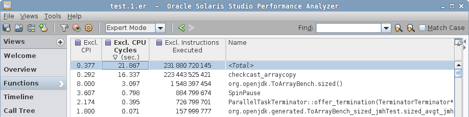
$ perfanal-hwc java -jar benchmarks.jar -f 1 -p size=1000 -p type=arraylist

This will create the test.${n}.er result file in your current directory, which you can then open with Analyzer GUI. The GUI is rich enough to understand intuitively, and here is what we see in it.

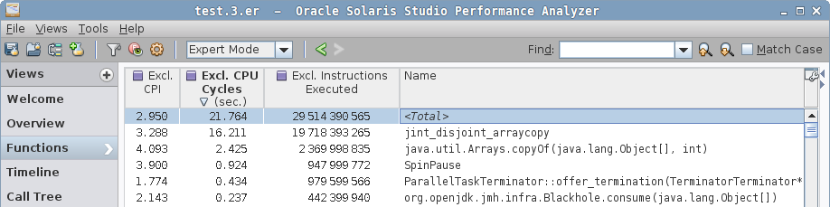
Figure 4. ArrayList (size = 1000), toArray().

In a simple case, we see the hottest function is jint_disjoint_arraycopy, which seems to be the function that implements an "int" arraycopy for disjoint arrays.

Note how the profiler resolved both Java code (org.openjdk…), VM native code (ParallelTaskTerminator::… and SpinPause), and generated VM stubs (e.g. jint_disjoint_arraycopy). In complex scenarios, call trees would show both Java and native frames, which is immensely helpful when debugging JNI/JNA cases, including calls into the VM itself.

The "Call Tree" would show you that this jint_disjoint_arraycopy is a leaf function. There is no other indication as to what this function is, but you can search around in Hotspot source base, then you will stumble upon stubRoutines.hpp, which will say that "StubRoutines provides entry points to assembly routines used by compiled code and the run-time system. Platform-specific entry points are defined in the platform-specific inner class." Both compiler and runtime use that to optimize some operations, notably arraycopy.

Figure 5. ArrayList (size = 1000), toArray(new T[list.size()]).

In a sized case, we see a different function for arraycopy, checkcast_arraycopy, plus the Java code for sized() method.

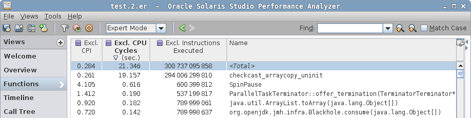
Figure 6. ArrayList (size = 1000), toArray(new T[0]).

In a zero case, we see yet another contender, checkcast_arraycopy_uninit, which looks like a modification of checkcast_arraycopy, but "uninitialized"? Notice the Java method is gone from hotspots.

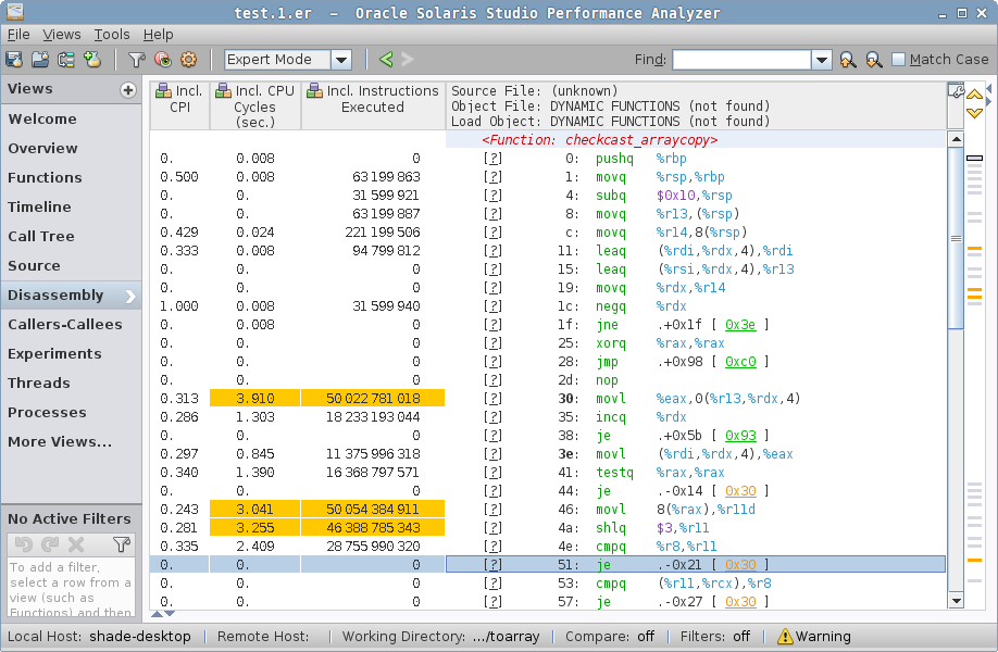
Well, the function names are already quite revealing, but it would be only an educated guess until we invoke another outstanding feature of Analyzer. If we select the function from the list (or "Call Tree"), and switch to "Disassembly" view, we will see… wait for it… disassembly!

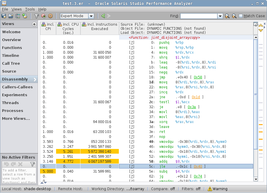
Figure 7. simple case disassembly.

The jint_disjoint_arraycopy is indeed the copying stub, which employs AVX for vectorized copy! No wonder this thing is fast: it copies the backing storage in large strides.

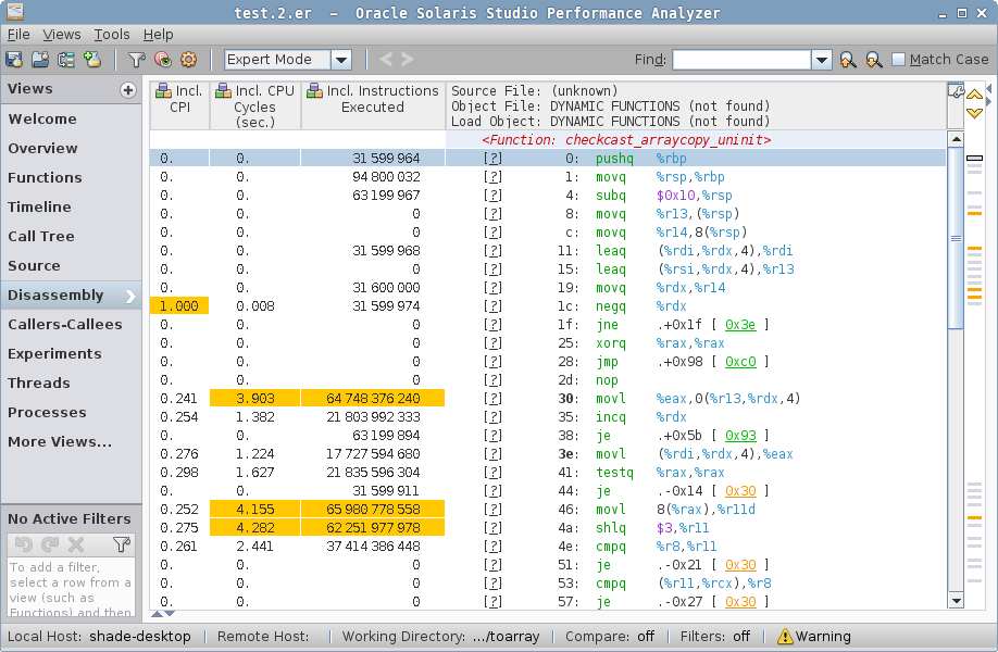
Figure 8. zero case disassembly

zero case disassembly shows non-vectorized checkcast_arraycopy_uninit. What does it do? The loop at relative addresses 30-51 is indeed copying, but it does not seem to be vectorized at all. Alas, deciphering what it does requires some VM internals knowledge. Normally, you will be able to attach the Java code to assembly, but VM stubs have no Java code associated with them. You can also trace the VM source code that generated the stub. Here, we will just stare patiently at the code.

The loop reads with movl(%rdi,%rdx,4),%eax and writes with movl %eax, 0(%r13,%rdx,4), and %rdx is increasing — it follows from that %rdx is the loop counter. After reading the current element to %eax, we null-check it, load something from offset 0x8, shift it, and compare with something else. That is loading a class word, unpacking it, and doing the typecheck against it.

You can peek around the runtime representation of Java Objects with JOL. Notably, see the JOLSample_11_ClassWord example.

Figure 9. sized case disassembly, arraycopy stub

sized has two hotspots, one in checkcast_arraycopy, where the hot loop is actually the same as in zero case above, but then we come to a second hotspot:

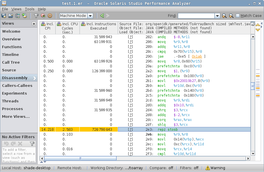
Figure 10. sized case disassembly, Java code

…which attributes most cycles to the repz stosb instruction. This is cryptic until you look around the generated code. prefetchnta instructions in HotSpot-generated code usually attributes to "allocation prefetch" (see command line docs, "-XX:Allocate…"), which is tied to object allocation. In fact, we have the "new" object address in %r9, and we put the mark word, class word, and then zero the storage with repz stosb — that’s a "memset to zero" in disguise. The allocation itself is an array allocation, and what we see is the array zeroing. You can read about this in greater detail in "Why Nothing Matters: The Impact of Zeroing".

Preliminaries

With that, we have our preliminary insights:

Vectorized arraycopy in the simple case is much faster than type-checked arraycopy in sized and zero.
Magically dodging the array zeroing lets zero become faster than sized. "Reflective" array creation does not seem to affect zero case at all.

Redoing the same for HashSet is left as the exercise to the reader: it will bring roughly the same preliminary answers.

Follow-Ups

In way too many cases, it is instructive and educational to follow up on the findings you just got from a targeted workload, in order to see how general the conclusions are, and whether you understand them well. Beware, this is the Rabbit Hole of Performance Engineering — you cannot finish the dive, you can only stop it.

New Reflective Array

First, let us deconstruct the "reflective array creation is slow" sentiment. We know that many collections instantiate the arrays of a given type with Array.newInstance(Class<?>,int) — why don’t we give it a try? Let’s see, having the same benchmarking ideas in mind, let us strip away everything except the newInstance call:

@Warmup(iterations = 10, time = 1, timeUnit = TimeUnit.SECONDS)
@Measurement(iterations = 10, time = 1, timeUnit = TimeUnit.SECONDS)
@Fork(value = 3, jvmArgsAppend = {"-XX:+UseParallelGC", "-Xms1g", "-Xmx1g"})
@BenchmarkMode(Mode.AverageTime)
@OutputTimeUnit(TimeUnit.NANOSECONDS)
@State(Scope.Benchmark)
public class ReflectiveArrayBench {

    @Param({"0", "1", "10", "100", "1000"})
    int size;

    @Benchmark
    public Foo[] lang() {
        return new Foo[size];
    }

    @Benchmark
    public Foo[] reflect() {
        return (Foo[]) Array.newInstance(Foo.class, size);
    }
}

Now, if you look into the performance data, you’ll notice that the performance is the same for both "language" expression for array instantiation and the reflective call:

Benchmark                     (size)  Mode  Cnt    Score    Error  Units

# default
ReflectiveArrayBench.lang          0  avgt    5   17.065 ±  0.224  ns/op
ReflectiveArrayBench.lang          1  avgt    5   12.372 ±  0.112  ns/op
ReflectiveArrayBench.lang         10  avgt    5   14.910 ±  0.850  ns/op
ReflectiveArrayBench.lang        100  avgt    5   42.942 ±  3.666  ns/op
ReflectiveArrayBench.lang       1000  avgt    5  267.889 ± 15.719  ns/op

# default
ReflectiveArrayBench.reflect       0  avgt    5   17.010 ±  0.299  ns/op
ReflectiveArrayBench.reflect       1  avgt    5   12.542 ±  0.322  ns/op
ReflectiveArrayBench.reflect      10  avgt    5   12.835 ±  0.587  ns/op
ReflectiveArrayBench.reflect     100  avgt    5   42.691 ±  2.204  ns/op
ReflectiveArrayBench.reflect    1000  avgt    5  264.408 ± 22.079  ns/op

Why is that? Where’s my expensive reflection call? To cut the chase short, you can usually do these steps to bisect this "oddity". First, google/remember that for a long time Reflection calls get "inflated" (the transition from JNI, which has larger per-call cost but avoids one-time setup, to faster JNI-free generated code once an invocation threshold is hit). Turn off Reflection inflation:

Benchmark                     (size)  Mode  Cnt    Score   Error  Units

# -Dsun.reflect.inflationThreshold=2147483647
ReflectiveArrayBench.reflect       0  avgt   10   17.253 ± 0.470  ns/op
ReflectiveArrayBench.reflect       1  avgt   10   12.418 ± 0.101  ns/op
ReflectiveArrayBench.reflect      10  avgt   10   12.554 ± 0.109  ns/op
ReflectiveArrayBench.reflect     100  avgt   10   39.969 ± 0.367  ns/op
ReflectiveArrayBench.reflect    1000  avgt   10  252.281 ± 2.630  ns/op

Hm, well, that’s not it. Let’s dig into the source code:

jdk/src/java.base/share/classes/java/lang/reflect/Array.java

class Array {
    public static Object newInstance(Class<?> componentType, int length)
        throws NegativeArraySizeException {
        return newArray(componentType, length);
    }

    @HotSpotIntrinsicCandidate // <--- Ohh, what's this?
    private static native Object newArray(Class<?> componentType, int length)
        throws NegativeArraySizeException;
}

jdk/src/java.base/share/classes/jdk/internal/HotSpotIntrinsicCandidate.java

/**
 * The {@code @HotSpotIntrinsicCandidate} annotation is specific to the
 * HotSpot Virtual Machine. It indicates that an annotated method
 * may be (but is not guaranteed to be) intrinsified by the HotSpot VM. A method
 * is intrinsified if the HotSpot VM replaces the annotated method with hand-written
 * assembly and/or hand-written compiler IR -- a compiler intrinsic -- to improve
 * performance. The {@code @HotSpotIntrinsicCandidate} annotation is internal to the
 * Java libraries and is therefore not supposed to have any relevance for application
 * code.
 */
public @interface HotSpotIntrinsicCandidate { ... }

So, the Array.newArray method is known to the VM. Interesting, let’s see under what name:

hotspot/src/share/vm/classfile/vmSymbols.hpp

  do_intrinsic(_newArray, java_lang_reflect_Array, newArray_name, newArray_signature, F_SN) \
   do_name(     newArray_name,       "newArray")                                            \
   do_signature(newArray_signature,  "(Ljava/lang/Class;I)Ljava/lang/Object;")              \

Intrinsic, eh? Let me try to disable you:

# -XX:+UnlockDiagnosticVMOptions -XX:DisableIntrinsic=_newArray
ReflectiveArrayBench.reflect       0  avgt    5   67.594 ± 4.795  ns/op
ReflectiveArrayBench.reflect       1  avgt    5   69.935 ± 7.766  ns/op
ReflectiveArrayBench.reflect      10  avgt    5   73.588 ± 0.329  ns/op
ReflectiveArrayBench.reflect     100  avgt    5   86.598 ± 1.735  ns/op
ReflectiveArrayBench.reflect    1000  avgt    5  409.786 ± 9.148  ns/op

Aha, there! This is handled specifically by the JVM, and the same generated code is emitted. But, don’t ever assume any "fancy" option you have seen on the Internet does what you think it does. Let us take the profile in Performance Analyzer:

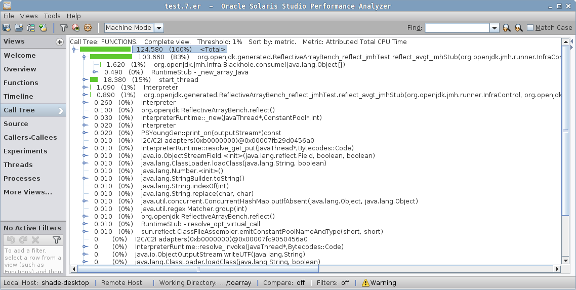
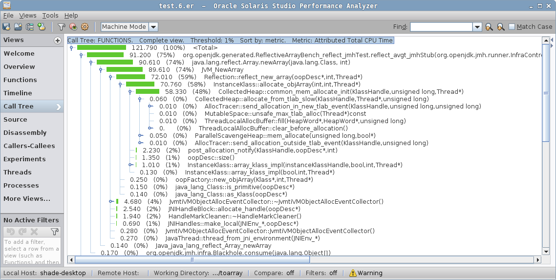
Figure 11. _newArray intrinsic enabled

Figure 12. _newArray intrinsic disabled

See the difference? When the intrinsic is disabled, we have the Java method for Array.newArray, then a call to the JVM_NewArray native method implementation, which then calls the VM’s Reflection::…, and goes from there to the GC asking to allocate the array. This must be what people have seen as an expensive "Array.newArray call".

But, that is not true anymore. JIRA archeology points at JDK-6525802 as the fix. We’ll explore historical performance data later.

Empty Array Instantiation

Now, let’s shift attention to array instantiation costs. It is important to understand how the allocation itself works before we jump to zeroing elimination. In hindsight, we would want to measure both constant sized arrays, and non-constant sized arrays where the array size is not statically known. Can the compiler do something with that knowledge?

Let’s see, and build the JMH benchmark like this (I describe it in a pseudo-macro-language to make it shorter):

@Warmup(iterations = 10, time = 1, timeUnit = TimeUnit.SECONDS)
@Measurement(iterations = 10, time = 1, timeUnit = TimeUnit.SECONDS)
@Fork(value = 3, jvmArgsAppend = {"-XX:+UseParallelGC", "-Xms1g", "-Xmx1g"})
@BenchmarkMode(Mode.AverageTime)
@OutputTimeUnit(TimeUnit.NANOSECONDS)
@State(Scope.Benchmark)
public class EmptyArrayBench {

#for L in 0..512
    int v$L = $L;

    @Benchmark
    public Foo[] field_$L() {
        return new Foo[v$L];
    }

    @Benchmark
    public Foo[] const_$L() {
        return new Foo[$L];
    }
#done
}

Running this benchmark would yield something like:

Benchmark                 Mode  Cnt   Score   Error  Units

# -----------------------------------------------------------

EmptyArrayBench.const_000  avgt   15    2.847 ± 0.016  ns/op
EmptyArrayBench.const_001  avgt   15    3.090 ± 0.020  ns/op
EmptyArrayBench.const_002  avgt   15    3.083 ± 0.022  ns/op
EmptyArrayBench.const_004  avgt   15    3.336 ± 0.029  ns/op
EmptyArrayBench.const_008  avgt   15    4.618 ± 0.047  ns/op
EmptyArrayBench.const_016  avgt   15    7.568 ± 0.061  ns/op
EmptyArrayBench.const_032  avgt   15   13.935 ± 0.098  ns/op
EmptyArrayBench.const_064  avgt   15   25.905 ± 0.183  ns/op
EmptyArrayBench.const_128  avgt   15   52.807 ± 0.252  ns/op
EmptyArrayBench.const_256  avgt   15  110.208 ± 1.006  ns/op
EmptyArrayBench.const_512  avgt   15  171.864 ± 0.777  ns/op

# -----------------------------------------------------------

EmptyArrayBench.field_000  avgt   15   16.998 ± 0.063  ns/op
EmptyArrayBench.field_001  avgt   15   12.400 ± 0.065  ns/op
EmptyArrayBench.field_002  avgt   15   12.651 ± 0.332  ns/op
EmptyArrayBench.field_004  avgt   15   12.434 ± 0.062  ns/op
EmptyArrayBench.field_008  avgt   15   12.504 ± 0.049  ns/op
EmptyArrayBench.field_016  avgt   15   12.588 ± 0.065  ns/op
EmptyArrayBench.field_032  avgt   15   14.423 ± 0.121  ns/op
EmptyArrayBench.field_064  avgt   15   26.145 ± 0.166  ns/op
EmptyArrayBench.field_128  avgt   15   53.092 ± 0.291  ns/op
EmptyArrayBench.field_256  avgt   15  110.275 ± 1.304  ns/op
EmptyArrayBench.field_512  avgt   15  174.326 ± 1.642  ns/op

# -----------------------------------------------------------

Oops. It would seem that field_* tests lose on small lengths. Why is that? -prof perfasm has a hint:

Hottest allocation code in const_0008:

  2.30%    1.07%  0x00007f32cd1f9f76: prefetchnta 0xc0(%r10)
  3.34%    3.88%  0x00007f32cd1f9f7e: movq   $0x1,(%rax)
  3.66%    4.39%  0x00007f32cd1f9f85: prefetchnta 0x100(%r10)
  1.63%    1.91%  0x00007f32cd1f9f8d: movl   $0x20018fbd,0x8(%rax)
  1.76%    2.31%  0x00007f32cd1f9f94: prefetchnta 0x140(%r10)
  1.52%    2.14%  0x00007f32cd1f9f9c: movl   $0x8,0xc(%rax)
  2.77%    3.67%  0x00007f32cd1f9fa3: prefetchnta 0x180(%r10)
  1.77%    1.80%  0x00007f32cd1f9fab: mov    %r12,0x10(%rax)
  4.40%    4.61%  0x00007f32cd1f9faf: mov    %r12,0x18(%rax)
  4.64%    3.97%  0x00007f32cd1f9fb3: mov    %r12,0x20(%rax)
  4.83%    4.49%  0x00007f32cd1f9fb7: mov    %r12,0x28(%rax)
  2.03%    2.71%  0x00007f32cd1f9fbb: mov    %r8,0x18(%rsp)
  1.35%    1.25%  0x00007f32cd1f9fc0: mov    %rax,%rdx

Hottest allocation code in field_0008:

  0.02%           0x00007f27551fb424: prefetchnta 0xc0(%r11)
  5.53%    7.55%  0x00007f27551fb42c: movq   $0x1,(%r9)
  0.02%           0x00007f27551fb433: prefetchnta 0x100(%r11)
  0.05%    0.06%  0x00007f27551fb43b: movl   $0x20018fbd,0x8(%r9)
           0.01%  0x00007f27551fb443: mov    %edx,0xc(%r9)
  2.03%    1.78%  0x00007f27551fb447: prefetchnta 0x140(%r11)
  0.04%    0.07%  0x00007f27551fb44f: mov    %r9,%rdi
  0.02%    0.02%  0x00007f27551fb452: add    $0x10,%rdi
  0.02%    0.01%  0x00007f27551fb456: prefetchnta 0x180(%r11)
  1.96%    1.05%  0x00007f27551fb45e: shr    $0x3,%rcx
  0.02%    0.02%  0x00007f27551fb462: add    $0xfffffffffffffffe,%rcx
  0.01%    0.03%  0x00007f27551fb466: xor    %rax,%rax
  0.01%           0x00007f27551fb469: shl    $0x3,%rcx
  1.96%    0.06%  0x00007f27551fb46d: rep rex.W stos %al,%es:(%rdi) ; <--- huh...
 39.44%   78.39%  0x00007f27551fb470: mov    %r8,0x18(%rsp)
  8.01%    0.18%  0x00007f27551fb475: mov    %r9,%rdx

Digging further, you would notice that even const_* cases switch back to rep stos after some threshold (pretty much how other memset implementations do), trying to dodge the setup costs of rep stos at low sizes. But field_* cases, not knowing the length statically, always do the rep stos, and are penalized on small lengths.

This is somewhat fixable, see JDK-8146801. However, constant sizes would be at least as better. Do you get how this applies to our toArray case? Compare new T[0] or new T[coll.size()] on small collection sizes. This answers where zero case gets a part of its "anomalous" advantage on small sizes.

This is another instance of "the more the compiler can assume about the code, the better it can optimize". Constants rule! A marginally more interesting case is described at "Faster Atomic*FieldUpdaters for Everyone".

Uninitialized Arrays

Now, to the "zeroing" part of the story. The Java Language specification requires that newly instantiated arrays and objects have default field values (zeroes), not some arbitrary values that were left over in the memory. For that reason, runtimes have to zero-out the allocated storage. However, if we overwrite that storage with some initial values before an object/array is visible to anything else, then we can coalesce the initialization with zeroing, effectively removing the zeroing. Note that "visible" can be tricky to define in the face of exceptional returns, finalizers, and other VM internals, see e.g. JDK-8074566.

We have seen that zero case had managed to avoid zeroing, but sized case did not. Is this an oversight? To explore that, we might want to evaluate different code where an array is allocated, and then a subsequent arraycopy overwrites its contents. Like this:

@Warmup(iterations = 10, time = 1, timeUnit = TimeUnit.SECONDS)
@Measurement(iterations = 10, time = 1, timeUnit = TimeUnit.SECONDS)
@Fork(value = 3, jvmArgsAppend = {"-XX:+UseParallelGC", "-Xms1g", "-Xmx1g"})
@BenchmarkMode(Mode.AverageTime)
@OutputTimeUnit(TimeUnit.NANOSECONDS)
@State(Scope.Benchmark)
public class ArrayZeroingBench {
    @Param({"1", "10", "100", "1000"})
    int size;

    Object[] src;

    @Setup
    public void setup() {
        src = new Object[size];
        for (int c = 0; c < size; c++) {
            src[c] = new Foo();
        }
    }

    @Benchmark
    public Foo[] arraycopy_base() {
        Object[] src = this.src;
        Foo[] dst = new Foo[size];
        System.arraycopy(src, 0, dst, 0, size - 1);
        return dst;
    }

    @Benchmark
    public Foo[] arraycopy_field() {
        Object[] src = this.src;
        Foo[] dst = new Foo[size];
        System.arraycopy(src, 0, dst, 0, size);
        return dst;
    }

    @Benchmark
    public Foo[] arraycopy_srcLength() {
        Object[] src = this.src;
        Foo[] dst = new Foo[size];
        System.arraycopy(src, 0, dst, 0, src.length);
        return dst;
    }

    @Benchmark
    public Foo[] arraycopy_dstLength() {
        Object[] src = this.src;
        Foo[] dst = new Foo[size];
        System.arraycopy(src, 0, dst, 0, dst.length);
        return dst;
    }

    @Benchmark
    public Foo[] copyOf_field() {
        return Arrays.copyOf(src, size, Foo[].class);
    }

    @Benchmark
    public Foo[] copyOf_srcLength() {
        return Arrays.copyOf(src, src.length, Foo[].class);
    }

    public static class Foo {}
}

Running this benchmark would yield some interesting results:

Benchmark                (size)  Mode  Cnt    Score    Error  Units
AZB.arraycopy_base            1  avgt   15   14.509 ±  0.066  ns/op
AZB.arraycopy_base           10  avgt   15   23.676 ±  0.557  ns/op
AZB.arraycopy_base          100  avgt   15   92.557 ±  0.920  ns/op
AZB.arraycopy_base         1000  avgt   15  899.859 ±  7.303  ns/op

AZB.arraycopy_dstLength       1  avgt   15   17.929 ±  0.069  ns/op
AZB.arraycopy_dstLength      10  avgt   15   23.613 ±  0.368  ns/op
AZB.arraycopy_dstLength     100  avgt   15   92.553 ±  0.432  ns/op
AZB.arraycopy_dstLength    1000  avgt   15  902.176 ±  5.816  ns/op

AZB.arraycopy_field           1  avgt   15   18.063 ±  0.375  ns/op
AZB.arraycopy_field          10  avgt   15   23.443 ±  0.278  ns/op
AZB.arraycopy_field         100  avgt   15   93.207 ±  1.565  ns/op
AZB.arraycopy_field        1000  avgt   15  908.663 ± 18.383  ns/op

AZB.arraycopy_srcLength       1  avgt   15    8.658 ±  0.058  ns/op
AZB.arraycopy_srcLength      10  avgt   15   14.114 ±  0.084  ns/op
AZB.arraycopy_srcLength     100  avgt   15   79.778 ±  0.639  ns/op
AZB.arraycopy_srcLength    1000  avgt   15  681.040 ±  9.536  ns/op

AZB.copyOf_field              1  avgt   15    9.383 ±  0.053  ns/op
AZB.copyOf_field             10  avgt   15   14.729 ±  0.091  ns/op
AZB.copyOf_field            100  avgt   15   81.198 ±  0.477  ns/op
AZB.copyOf_field           1000  avgt   15  671.670 ±  6.723  ns/op

AZB.copyOf_srcLength          1  avgt   15    8.150 ±  0.409  ns/op
AZB.copyOf_srcLength         10  avgt   15   13.214 ±  0.112  ns/op
AZB.copyOf_srcLength        100  avgt   15   80.718 ±  1.583  ns/op
AZB.copyOf_srcLength       1000  avgt   15  671.716 ±  5.499  ns/op

Of course, you need to study the generated code to validate any hypothesis about these results, and in fact we did in JDK-8146828. VM tries to eliminate as much zeroing as it could, because the optimization is quite profitable — this is why zero case (which is similar to copyOf_*) code shape benefits.

But in some cases, the code shape is not recognized as a "tightly coupled" allocation, and zeroing is not removed, which should be fixed, see JDK-8146828.

Caching the Array

Many can ask another follow-up: given that zero is well-optimized, can we push the envelope further and use the static constant with zero-sized array to convey the type information? With that, we might be able to avoid the stray allocation completely? Let’s see, and add zero_cached test:

@State(Scope.Benchmark)
public class ToArrayBench {

    // Note this is *both* static *and* final
    private static final Foo[] EMPTY_FOO = new Foo[0];

    ...

    @Benchmark
    public Foo[] zero() {
        return coll.toArray(new Foo[0]);
    }

    @Benchmark
    public Foo[] zero_cached() {
        return coll.toArray(EMPTY_FOO);
    }
}

Note that these cases are subtly different: for empty collections, zero_cached would return the same array, not a distinct array for each call. This may be problematic if users are using array identity for something, and this pretty much invalidates the hope for doing this substitution everywhere, and automatically.

Running this benchmark would yield:

Benchmark               (size)     (type)  Mode  Cnt     Score    Error  Units

# ----------------------------------------------------------------------------

ToArrayBench.zero            0  arraylist  avgt   15     4.352 ±  0.034  ns/op
ToArrayBench.zero            1  arraylist  avgt   15    10.574 ±  0.075  ns/op
ToArrayBench.zero           10  arraylist  avgt   15    15.965 ±  0.166  ns/op
ToArrayBench.zero          100  arraylist  avgt   15    81.729 ±  0.650  ns/op
ToArrayBench.zero         1000  arraylist  avgt   15   685.616 ±  6.637  ns/op

ToArrayBench.zero_cached     0  arraylist  avgt   15     4.031 ±  0.018  ns/op
ToArrayBench.zero_cached     1  arraylist  avgt   15    10.237 ±  0.104  ns/op
ToArrayBench.zero_cached    10  arraylist  avgt   15    15.401 ±  0.903  ns/op
ToArrayBench.zero_cached   100  arraylist  avgt   15    82.643 ±  1.040  ns/op
ToArrayBench.zero_cached  1000  arraylist  avgt   15   688.412 ± 18.273  ns/op

# ----------------------------------------------------------------------------

ToArrayBench.zero            0    hashset  avgt   15     4.382 ±  0.028  ns/op
ToArrayBench.zero            1    hashset  avgt   15    23.877 ±  0.139  ns/op
ToArrayBench.zero           10    hashset  avgt   15    44.172 ±  0.353  ns/op
ToArrayBench.zero          100    hashset  avgt   15   282.852 ±  1.372  ns/op
ToArrayBench.zero         1000    hashset  avgt   15  4370.370 ± 64.018  ns/op

ToArrayBench.zero_cached     0    hashset  avgt   15     3.525 ±  0.005  ns/op
ToArrayBench.zero_cached     1    hashset  avgt   15    23.791 ±  0.162  ns/op
ToArrayBench.zero_cached    10    hashset  avgt   15    44.128 ±  0.203  ns/op
ToArrayBench.zero_cached   100    hashset  avgt   15   282.052 ±  1.469  ns/op
ToArrayBench.zero_cached  1000    hashset  avgt   15  4329.551 ± 36.858  ns/op

# ----------------------------------------------------------------------------

As expected, the only effect whatsoever can be observed on a very small collection sizes, and this is only a marginal improvement over new Foo[0]. This improvement does not seem to justify caching the array in the grand scheme of things. As a teeny tiny micro-optimization, it might make sense in some tight code, but I wouldn’t care otherwise.

Historical Perspective

Now, a little backtracking to see how the original benchmark performs on different historical JDKs. JMH benchmarks can run with anything starting with JDK 6. /me blows some dust from JDK releases archive. Let’s poke at a few interesting points in JDK 6’s lifetime, and also see how the latest JDK 8u66 and JDK 9b99 performs.

We don’t need all the sizes, just consider some reasonable size:

Benchmark            (size)     (type)  Mode  Cnt    Score   Error  Units

# --------------------------------------------------------------------------

# 6u6 (2008-04-16)
ToArrayBench.simple     100  arraylist  avgt   30  122.228 ± 1.413  ns/op
ToArrayBench.sized      100  arraylist  avgt   30  139.403 ± 1.024  ns/op
ToArrayBench.zero       100  arraylist  avgt   30  155.176 ± 3.673  ns/op

# 6u12 (2008-12-12)
ToArrayBench.simple     100  arraylist  avgt   30   84.760 ± 1.283  ns/op
ToArrayBench.sized      100  arraylist  avgt   30  142.400 ± 2.696  ns/op
ToArrayBench.zero       100  arraylist  avgt   30   94.132 ± 0.636  ns/op

# 8u66 (2015-11-16)
ToArrayBench.simple     100  arraylist  avgt   30   41.174 ± 0.953  ns/op
ToArrayBench.sized      100  arraylist  avgt   30   93.159 ± 0.368  ns/op
ToArrayBench.zero       100  arraylist  avgt   30   80.193 ± 0.362  ns/op

# 9b99 (2016-01-05)
ToArrayBench.simple     100  arraylist  avgt   30   40.874 ± 0.352  ns/op
ToArrayBench.sized      100  arraylist  avgt   30   93.170 ± 0.379  ns/op
ToArrayBench.zero       100  arraylist  avgt   30   80.966 ± 0.347  ns/op

# --------------------------------------------------------------------------

# 6u12 (2008-12-12)
ToArrayBench.simple     100    hashset  avgt   30  585.766 ± 5.946  ns/op
ToArrayBench.sized      100    hashset  avgt   30  670.119 ± 0.959  ns/op
ToArrayBench.zero       100    hashset  avgt   30  745.802 ± 5.309  ns/op

# 6u16 (2009-08-11)
ToArrayBench.simple     100    hashset  avgt   30  561.724 ± 5.094  ns/op
ToArrayBench.sized      100    hashset  avgt   30  634.155 ± 0.557  ns/op
ToArrayBench.zero       100    hashset  avgt   30  634.300 ± 1.206  ns/op

# 6u21 (2010-07-07)
ToArrayBench.simple     100    hashset  avgt   30  565.139 ± 3.763  ns/op
ToArrayBench.sized      100    hashset  avgt   30  623.901 ± 4.027  ns/op
ToArrayBench.zero       100    hashset  avgt   30  605.833 ± 2.909  ns/op

# 8u66 (2015-11-16)
ToArrayBench.simple     100    hashset  avgt   30  297.281 ± 1.258  ns/op
ToArrayBench.sized      100    hashset  avgt   30  387.633 ± 0.787  ns/op
ToArrayBench.zero       100    hashset  avgt   30  307.410 ± 6.981  ns/op

# 9b99 (2016-01-05)
ToArrayBench.simple     100    hashset  avgt   30  298.032 ± 3.925  ns/op
ToArrayBench.sized      100    hashset  avgt   30  316.250 ± 9.614  ns/op
ToArrayBench.zero       100    hashset  avgt   30  284.431 ± 6.201  ns/op

# --------------------------------------------------------------------------

So, zero has been faster than sized for at least 5 years now.

Also notice how performance improves as the JDK improves. Way too often "Java is slow" is heard from people stuck on outdated JVMs. Update! (Although there are some real and not-yet-resolved performance problems. Only new and overhyped platforms don’t have problems, because nobody cares enough yet to discover them)

Conclusion

Putting it all together, we can promote our preliminary insights to actual conclusions:

Reflective array creation performance does not affect toArray(new T[0]) case at all, because Arrays.newArray is handled well by current VMs. Therefore, the premise for PMD’s and IDEA’s static analysis rule is invalid today. This is the first-order effect at play here, the rest is the difference between the different toArray implementation details.
Vectorized arraycopy in the Object[] toArray() case is much faster than the type-checked arraycopy in toArray(new T[size]) and toArray(new T[0]). Alas, that does not help us if we want to get T[].
A significant part of difference between toArray(new T[size]) and toArray(new T[0]) on small arrays lies in the ability to predict size, which maybe because size is loaded from a constant, comes from a statically known expression, or involves some other arcane magic. When size() is polled out of the collection itself, we would need to successfully inline the method, and hope the method is O(1). To add insult to injury, if the collection size had changed between polling size() and calling toArray(), we are so royally screwed.
But an even more significant part of toArray(new T[size]) vs toArray(new T[0]) story is zeroing elimination, which is predicated on VM’s ability to figure out that a newly-allocated array is fully populated. Current experiments show that at least for ArrayList cases, internally allocated array is faster because of that, and there is a chance for the externally allocated array to piggyback on the same mechanism. Some caveats on size from the previous bullet are relaxed, if we can completely eliminate the zeroing.

Bottom line: toArray(new T[0]) seems faster, safer, and contractually cleaner, and therefore should be the default choice now. Future VM optimizations may close this performance gap for toArray(new T[size]), rendering the current "believed to be optimal" usages on par with an actually optimal one. Further improvements in toArray APIs would follow the same logic as toArray(new T[0]) — the collection itself should create the appropriate storage.

Parting Thoughts

Performance suggestions are funny things. Their shelf life is limited, especially if you do not understand the background for them and don’t bother to track how the world evolves. Their applicability is frequently questionable, and many suggestions do not have a track to verify the experimental results. That’s why, if you really want peak performance, you have to allocate a dedicated set of persons who are well-versed in vetting the performance advice for you.

But, most of the time, the straight-forward code is fast enough, so stop philosophizing about angels on the head of a pin, and get back to work. 99.9% of applications do not need a dedicated team of performance engineers; they need instead for their developers to focus on writing clear, maintainable code, and a little bit of measurement and tuning to file off the rough edges when the code fails to meet the performance requirements.

That sane development practice sometimes gets contaminated when a longtime performance lore (e.g. "call toArray() with a pre-sized array") gets baked into tools, and becomes available as "quick hints" that turn out to be more of a nuisance, or even a right-away pessimisation.